QuTiP: Quantum Toolbox in Python

I was recently introduced to the quantum optics toolbox in Matlab, written by Sze Meng Tan, which is useful for quickly programming and studying a variety of quantum optics systems. Despite being great, the toolbox has not been updated since 2002.

Now there is QuTiP, a quantum toolbox for Python that is inspired by Sze's work. This software is actively maintained, and comes with a number of useful features. It is easy to parallelize certain tasks, it is more memory efficient, and it is faster. This toolbox has motivated me to learn Python–a surprisingly easy task. The excellent NumPy and Scipy libraries, along with Matplotlib, replicate most of the functionality found in Matlab with a similar syntax. A convenient way to install Python and the libraries that QuTip needs is to grab a copy of the Enthough Python Distribution, or if you already have Python installed to grab the Scipy Superpack. Note: QuTiP is only supported on Unix based systems like Linux or Mac OS X.

What makes this toolbox so great is that it allows you to write programs in a way that mimics how we write out physics problems. The program has lots of built in quantum opjects, such as annihilation, creation, squeezing, and displacement operators, that allow one to write down a Hamiltonian directly. Wigner and Q functions are built in, making it easy to plot quasi-probability distributions.

For example, this is the code used to create a coherent state.

N= 20 #Size of Hilbert Space 
alpha= 3 #amplitude of the coherent state 
D = displace(N,alpha) # Displacement operator 
vac= basis(N,0).unit() # Vacuum state 
psi=(D*vac).unit() # create a coherent state. The unit() ensures normalization.

It is easy to great operators as well. For example, let's look at how to create the nonstandard squeezing operator \(S3=\frac{1}{2}(\zeta^{\ast} a^{\dagger 3} - \zeta a^3),\) where \(\zeta\) is a squeezing parameter and \(a \) is the annihilation operator.

a = destroy(N) #annihilation operator 
S3=(1/2.0)*conj(zeta)*(a**3)-(1/2.0)*zeta*(a.dag())**3

Note: in Python ** means raise to the exponent. Here a**3 means \(a^3\).

QuTiP stores our operator as an object. One of the built-in methods allows us to exponentiate this operator so we can act on a state. For example, to create a squeezed state we act on the vacuum state with our squeezing operator, S3, and our displacement operator, D.

psi=(D*S3.expm()*vac).unit()

There is an impressive array of examples available from the QuTip website. The authors also have this paper that outlines how the program works, the performance benefits, and some excellent examples.

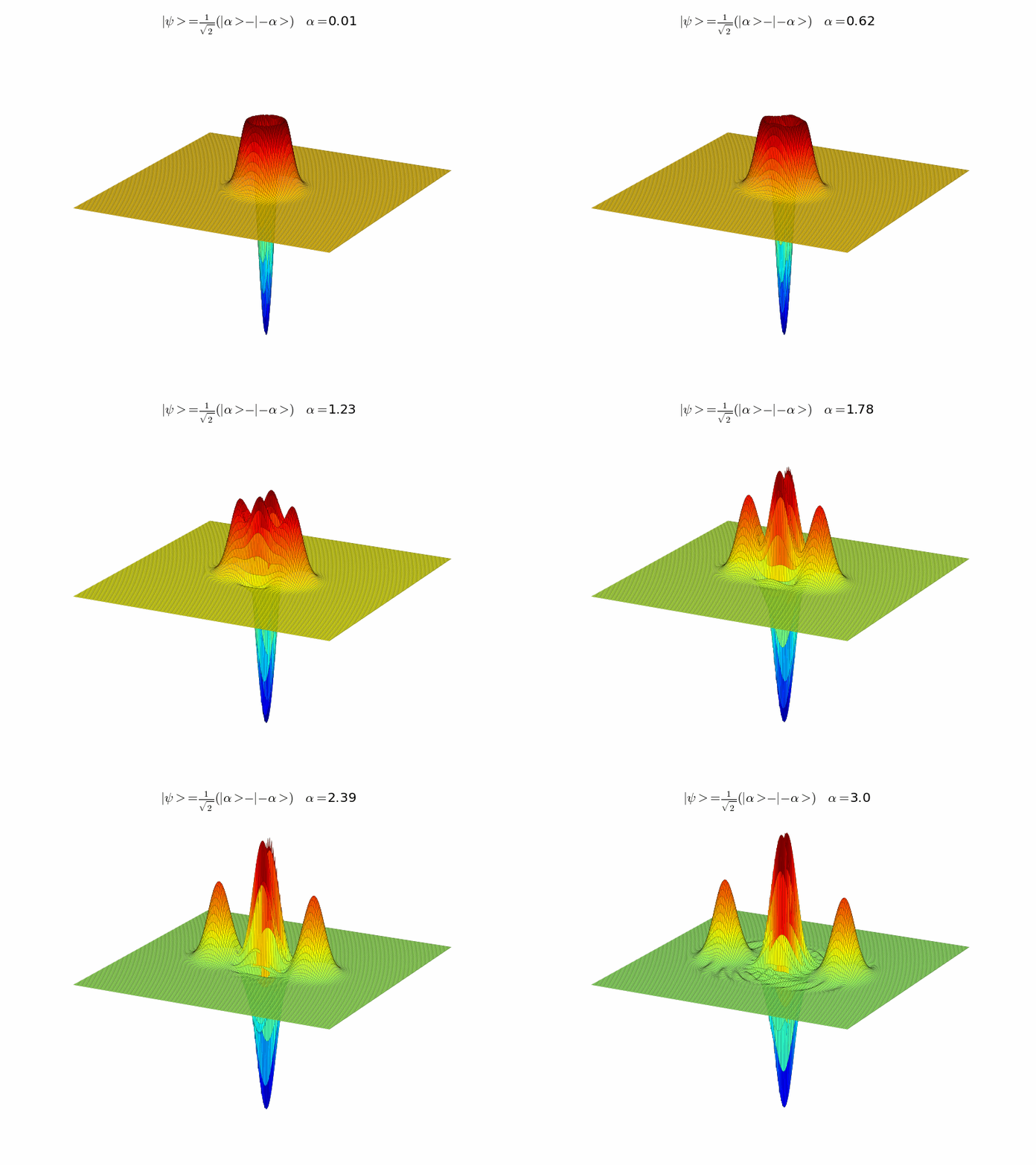
Here is a simple program I wrote, based on this example in the documentation, to plot the Wigner functions for a series of Schrödinger's cat states (a superposition of two different coherent states). The results are shown in the animated gif below.

# 3D Wigner functions for a series of cat states. #   
from qutip.states import *   
from qutip.Qobj import *   
from qutip.operators import *   
from qutip.wigner import *   
from mpl_toolkits.mplot3d import Axes3D   
from matplotlib import cm   
from pylab import *  

#setup constants: 
N = 20 # size of the Hilbert space 
alpha=linspace(0.01,3,60) # values for the coherent state amplitude 
a = destroy(N) #annihilation operator 
D = displace(N,alpha) # Displacement 
xvec = linspace(-9,9,300) 
X,Y = meshgrid(xvec, xvec)

k=1 # counter 
for x in alpha: 

    # Define the cat state. It is a coherent superposition of two coherent states. 
    # Each coherent state is created by the displacement operator acting on the vacuum. 
    # the unit() function makes sure that the overall state is normalized. 

    psi=(displace(N,x)*basis(N,0)-displace(N,-1*x)*basis(N,0)).unit();

    # plot the wigner function 
    W=wigner(psi,xvec,xvec) 
    fig =figure() 
    ax = Axes3D(fig,azim=-62.5,elev=25) 
    ax.plot_surface(X, Y, W, rstride=2, cstride=2, cmap=cm.jet,lw=.1) 
    ax.set_xlim3d(-9,9) 
    ax.set_xlim3d(-9,9) 
    ax.set_zlim3d(-.2,0.2) 
    ax.set_axis_off() 
    ax.set_frame_on('false') 
    title(r'$| \psi >= \frac{1}{\sqrt{2}}(|\alpha>-|-\alpha>)$'+r' $\alpha=$'+str(round(x,2))) 
    savefig("cat_state_"+str(k)+".png") k=k+1;

UPDATE: While I was writing this post, version 2 of QuTiP was released. I haven't had a chance to look at the new version in depth, but this looks like a solid update.